

Spin wave dispersion in a magnetic nanopillar with Ubermag
Published:
Spin waves — collective precessions of the magnetization in ordered magnetic materials — are at the heart of a rapidly growing field called magnonics: using magnons (the quanta of spin waves) to carry and process information. Unlike electrons, magnons carry no charge, so magnonic devices are free of Joule heating. Unlike photons, magnons have wavelengths in the nanometer range and can be confined to nanoscale waveguides.
This tutorial shows how to simulate spin wave propagation along a Permalloy nanowire using Ubermag, a Python interface to OOMMF. We follow the setup of the classic nmag nanopillar probe example introduced by Kruglyak, Dvornik, and Dmytriiev, implemented entirely in Python with Jupyter notebooks.
The strategy is a standard one in computational magnonics:
- Relax the wire to its equilibrium magnetization state.
- Strike one end with a short, spatially-localized magnetic field pulse.
- Record how the transverse magnetization \(\delta m_y(x,t)\) evolves along the wire.
- Apply a 2D Fourier transform to directly read off the dispersion relation \(\omega(k)\).
The full notebooks are in the repository: 03a_nanopillar.ipynb (simulation) and 03b_np_data.ipynb (data analysis).
1. The physics of micromagnetism
1.1 The magnetization field and length scales
In a ferromagnet, the magnetic moments of the electrons are exchange-coupled and align collectively below the Curie temperature, forming a spontaneous magnetization \(\mathbf{M}(\mathbf{r}, t)\). Micromagnetism is the continuum theory valid on length scales from a few nanometers up to a few micrometers — too large for atomistic spin models, too small for macroscopic magnetostatics.
The key constraint is that the magnitude of the magnetization is fixed:
\[|\mathbf{M}(\mathbf{r}, t)| = M_s \quad \text{everywhere inside the material}\]where \(M_s\) is the saturation magnetization. The magnetization can only rotate, never shrink or grow. It is therefore most natural to work with the normalized vector \(\mathbf{m} = \mathbf{M}/M_s \in S^2\).
The most important intrinsic length scale is the exchange length:
\[\ell_\text{ex} = \sqrt{\frac{2A}{\mu_0 M_s^2}}\]It measures how far the exchange stiffness \(A\) can maintain uniform magnetization against the demagnetizing field. For our Permalloy parameters (\(A = 13 \, \text{pJ/m}\), \(M_s = 0.86 \, \text{MA/m}\)):
\[\ell_\text{ex} = \sqrt{\frac{2 \times 13 \times 10^{-12}}{4\pi \times 10^{-7} \times (0.86 \times 10^6)^2}} \approx 5.3 \, \text{nm}\]Any feature in \(\mathbf{m}\) that varies on a scale shorter than \(\ell_\text{ex}\) costs enormous exchange energy and is strongly suppressed. This sets a minimum cell size for our numerical mesh: we must resolve \(\ell_\text{ex}\).
1.2 Energy terms
The total micromagnetic free energy has three contributions for our system:
Exchange energy — penalizes any spatial variation of \(\mathbf{m}\):
\[E_\text{ex} = A \int_V |\nabla \mathbf{m}|^2 \, dV\]The exchange stiffness \(A\) encodes the quantum-mechanical tendency of neighboring spins to stay parallel. A large \(A\) means the magnetization is stiff and resists twisting — spin waves are expensive to excite and have a steep (stiff) dispersion.
Demagnetization (magnetostatic) energy — long-range dipolar interaction:
\[E_\text{demag} = -\frac{\mu_0}{2} \int_V \mathbf{M} \cdot \mathbf{H}_\text{demag} \, dV\]The demagnetizing field \(\mathbf{H}_\text{demag}\) is generated by the divergence of \(\mathbf{M}\) (magnetic “charges”) and acts to close flux lines inside the body. It is the most computationally expensive term because it involves a convolution over all space.
For our thin, elongated wire aligned along \(x\), the demagnetizing tensor is highly anisotropic. The longitudinal demagnetizing factor \(N_x \approx 0\) (the wire does not oppose magnetization along its own axis), while the transverse factors \(N_y = N_z \approx 1/2\) (a circular cross-section splits the flux equally in \(y\) and \(z\)). This shape anisotropy strongly favors magnetization along \(x\) — it is the reason the equilibrium state is a nearly uniform magnetization along the wire axis.
Zeeman energy — coupling to an externally applied field \(\mathbf{H}_\text{ext}\):
\[E_Z = -\mu_0 M_s \int_V \mathbf{m} \cdot \mathbf{H}_\text{ext} \, dV\]We use this only during the pulse phase to perturb the magnetization. There is no static external bias field in this simulation.
1.3 The Landau–Lifshitz–Gilbert equation
The time evolution of \(\mathbf{m}\) is governed by the Landau–Lifshitz–Gilbert (LLG) equation:
\[\frac{d\mathbf{m}}{dt} = -\gamma_0 \, \mathbf{m} \times \mathbf{H}_\text{eff} + \alpha \, \mathbf{m} \times \frac{d\mathbf{m}}{dt}\]The first term is the precession: in an effective field \(\mathbf{H}_\text{eff}\), the magnetization precesses around the field axis at the Larmor frequency \(\omega_L = \gamma_0 |\mathbf{H}_\text{eff}|\), where \(\gamma_0 = \mu_0 \gamma = 2.211 \times 10^5 \, \text{m A}^{-1} \text{s}^{-1}\) is the gyromagnetic ratio.
The second term is the Gilbert damping: it acts perpendicular to both \(\mathbf{m}\) and \(d\mathbf{m}/dt\), spiraling the magnetization toward the effective field direction and dissipating energy. The dimensionless constant \(\alpha\) controls the rate:
- \(\alpha \to 0\): undamped precession, spin waves propagate forever.
- \(\alpha = 0.5\): heavy overdamping, the system relaxes exponentially to equilibrium with no oscillations. Ideal for energy minimization.
- \(\alpha = 0.05\): light damping, spin waves can propagate tens to hundreds of nanometers before decaying. Realistic for Permalloy.
The effective field is derived from the total energy as a functional derivative:
\[\mathbf{H}_\text{eff} = -\frac{1}{\mu_0 M_s} \frac{\delta E}{\delta \mathbf{m}} = \underbrace{\frac{2A}{\mu_0 M_s} \nabla^2 \mathbf{m}}_{\text{exchange}} + \underbrace{\mathbf{H}_\text{demag}}_{\text{magnetostatic}} + \underbrace{\mathbf{H}_\text{ext}}_{\text{Zeeman}}\]2. Spin waves in a nanowire: analytical theory
2.1 Linearization and plane waves
Consider the equilibrium state \(\mathbf{m}_0 = \hat{x}\) (uniform magnetization along the wire). A small transverse perturbation \(\delta\mathbf{m} = (\delta m_x, \delta m_y, \delta m_z)\) with \(|\delta\mathbf{m}| \ll 1\) is excited by the pulse. Since \(\mathbf{m}\) is a unit vector, the longitudinal component is second-order small: \(\delta m_x \approx -\frac{1}{2}(|\delta m_y|^2 + |\delta m_z|^2) \approx 0\).
The perturbation propagates along \(x\) as a plane wave:
\[\delta m_y(x,t) = u \, e^{i(kx - \omega t)}, \qquad \delta m_z(x,t) = v \, e^{i(kx - \omega t)}\]Substituting into the linearized LLG (with \(\alpha = 0\)) gives the spin wave eigenvalue problem.
2.2 Dispersion relation
For an infinite thin wire magnetized along \(x\) with no external bias field, and in the exchange-dominated regime (\(k \ell_\text{ex} \gg 1\), i.e., short wavelengths), the dispersion simplifies to:
\[\boxed{\omega(k) \approx \frac{2A\gamma_0}{\mu_0 M_s} k^2 = \frac{D}{\hbar} k^2}\]where \(D = 2A\gamma_0 / (\mu_0 M_s)\) is the spin wave stiffness. This quadratic \(k^2\) dispersion is the hallmark of exchange spin waves — analogous to the dispersion of a non-relativistic quantum particle (\(E = \hbar^2 k^2 / 2m\)), with the exchange length playing the role of a magnetic Bohr radius.
Including the magnetostatic corrections for a finite-radius wire (in the dipole-exchange regime, where both exchange and demagnetization matter), the dispersion at small \(k\) acquires a gap and a more complex structure. For a thin wire with circular cross-section of radius \(R\):
\[\omega^2(k) = \left[\omega_0 + \omega_M \frac{2A}{\mu_0 M_s^2} k^2\right] \left[\omega_0 + \omega_M \frac{2A}{\mu_0 M_s^2} k^2 + \omega_M F(kR)\right]\]where \(\omega_M = \gamma_0 \mu_0 M_s\), \(\omega_0 = \gamma_0 \mu_0 H_0\) (bias field, zero here), and \(F(kR)\) is a form factor encoding the magnetostatic profile across the cross-section. In the short-wavelength limit \(kR \gg 1\), \(F \to 0\) and we recover the pure exchange result above. In our simulation (\(R = 3 \, \text{nm}\), \(\ell_\text{ex} = 5.3 \, \text{nm}\)), the wire is only slightly thinner than the exchange length, so we are in a mixed regime and the full numerical result from OOMMF is the most reliable.
2.3 Group velocity and propagation
The group velocity of spin wave packets is:
\[v_g = \frac{d\omega}{dk} \approx \frac{4A\gamma_0}{\mu_0 M_s} k\]It vanishes at \(k = 0\) (standing-wave-like oscillation of the whole wire) and increases linearly with \(k\). This means shorter-wavelength magnons travel faster — the opposite of light, and qualitatively similar to water ripples. In our 600 nm wire and 200 ps simulation window, we can resolve group velocities from zero up to several km/s.
The spin wave attenuation length (distance over which the amplitude decays by \(1/e\)) is related to damping by \(\lambda_\text{att} = v_g / (\alpha \omega)\). With \(\alpha = 0.05\) and a typical frequency of 100 GHz, a magnon at \(k = 0.3 \, \text{rad/nm}\) (group velocity \(\approx 3 \, \text{km/s}\)) travels \(\sim 500 \, \text{nm}\) before decaying — just long enough to traverse the wire and reflect, which is exactly what we observe.
3. The system: Permalloy nanopillar
3.1 Why Permalloy?
Permalloy (Py, composition Fe\(_{20}\)Ni\(_{80}\)) is the workhorse material of micromagnetics. Its appeal for spin wave research comes from a combination of properties:
| Property | Value | Significance |
|---|---|---|
| Saturation magnetization \(M_s\) | \(0.86 \, \text{MA/m}\) | Strong magnonic signal |
| Exchange stiffness \(A\) | \(13 \, \text{pJ/m}\) | \(\ell_\text{ex} \approx 5.3 \, \text{nm}\) |
| Gilbert damping \(\alpha\) | \(0.005\)–\(0.02\) (bulk) | Spin waves propagate long distances |
| Magnetocrystalline anisotropy | Negligible | Clean, geometry-dominated physics |
| Coercivity | Near zero | Easy to saturate and reset |
The nearly-zero magnetocrystalline anisotropy means the magnetic behavior is almost entirely determined by the geometry (shape anisotropy), making Permalloy ideal for testing theoretical models. We use a slightly elevated damping (\(\alpha = 0.05\)) for the dynamics to keep the simulation time short while still resolving several bounces of the spin wave packet.
3.2 Geometry
The nanopillar is a cylinder of radius \(r = 3 \, \text{nm}\) and length \(l = 600 \, \text{nm}\), oriented along the \(x\)-axis. Its cross-sectional diameter (6 nm) is slightly larger than the exchange length (5.3 nm), placing us in a regime where the wire behaves almost as a 1D spin wave waveguide but with small transverse corrections.
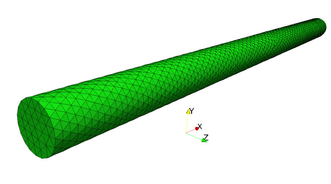 The nanopillar: a Permalloy cylinder of radius 3 nm and length 600 nm, aligned along the x-axis. The magnetization at equilibrium points uniformly along x (blue arrows). The pulse is applied at the left face (red region).
The aspect ratio \(l/r = 200\) ensures that the demagnetizing factor along \(x\) is negligible (\(N_x \approx 0\)), so there is essentially no shape-induced anisotropy opposing magnetization along the wire axis. This is why the ground state is a uniform single-domain state — no domain walls form.
4. Simulation — Part I: Setting up the system
4.1 Python packages
import discretisedfield as df   # geometry, mesh, and field objects
import micromagneticmodel as mm  # energy and dynamics terms (LLG)
import oommfc as mc              # drive OOMMF as a solver backend

import numpy as np
import ipywidgets as widgets
from IPython.display import display
Ubermag works as a Python frontend that constructs OOMMF’s .mif configuration files, runs OOMMF as a subprocess, and loads the results back into Python objects. You get the full power of OOMMF’s solver (adaptive time-stepping, mature magnetostatics solver) with a clean, Pythonic API.
4.2 Material parameters
Ms    = 0.86e6   # saturation magnetization (A/m)
A     = 13e-12   # exchange stiffness (J/m)
alpha = 0.5      # Gilbert damping — high for fast relaxation
The high damping (\(\alpha = 0.5\)) is used only during the energy minimization step. Physically, it means the precession term is heavily suppressed and the magnetization spirals to its equilibrium in the shortest possible simulation time.
4.3 Computational mesh
region = df.Region(p1=(-300e-9, -3e-9, -3e-9), p2=(300e-9, 3e-9, 3e-9))
mesh   = df.Mesh(region=region, cell=(3e-9, 1e-9, 1e-9))
The bounding box spans \(600 \times 6 \times 6 \, \text{nm}^3\). The cell size \(\Delta x \times \Delta y \times \Delta z = 3 \times 1 \times 1 \, \text{nm}^3\) is chosen with care:
- Along \(x\): \(\Delta x = 3 \, \text{nm} < \ell_\text{ex} = 5.3 \, \text{nm}\) — required to resolve exchange-driven magnetization variations. The cell also sets the shortest spatial wavelength resolvable: \(\lambda_\text{min} = 2\Delta x = 6 \, \text{nm}\), giving a Nyquist wavevector of \(k_\text{max} = \pi/\Delta x \approx 1.05 \, \text{rad/nm}\).
- Along \(y, z\): \(\Delta y = \Delta z = 1 \, \text{nm}\) — finer than the exchange length to correctly resolve the cross-sectional magnetostatic profile through the 6 nm diameter.
- Total cells: \(200 \times 6 \times 6 = 7200\). Small enough for fast single-machine runs.
4.4 Cylindrical geometry via a spatially-varying \(M_s\)
OOMMF uses rectangular meshes. We carve out the cylinder by defining \(M_s\) as a function of position: it returns the physical saturation magnetization inside the cylinder and zero outside. Cells with zero norm are excluded from all physics.
def Ms_fun(point):
    """Return Ms inside the cylinder (y² + z² < r²), 0 outside."""
    x, y, z = point
    if (y**2 + z**2)**0.5 < 3e-9:
        return Ms
    else:
        return 0
The argument valid="norm" in the field constructor below tells Ubermag/OOMMF that the valid simulation region is precisely the set of cells where norm > 0:
sys_relax = mm.System(name='nanopillar_relax_05')
sys_relax.m = df.Field(mesh, nvdim=3, value=(1, 0, 0), norm=Ms_fun, valid="norm")
nvdim=3: the field has three vector components \((m_x, m_y, m_z)\).value=(1, 0, 0): initial direction uniformly along \(x\).norm=Ms_fun: each cell’s magnitude is set toMs_fun(cell_center).
5. Simulation — Part II: Relaxation to equilibrium
5.1 Energy and dynamics for relaxation
We include only exchange and demagnetization — no applied field:
sys_relax.energy   = mm.Exchange(A=A) + mm.Demag()
sys_relax.dynamics = mm.Damping(alpha=alpha) + mm.Precession(gamma0=mm.consts.gamma0)
The dynamics are deliberately overdamped (\(\alpha = 0.5\)). At this damping, the precession is still present (we need it for the LLG to be well-posed) but the spiraling toward equilibrium dominates. The system reaches its ground state without overshooting.
5.2 Energy minimization
md = mc.MinDriver()
md.drive(sys_relax, dirname='../../data/simulations/')
MinDriver implements OOMMF’s conjugate-gradient energy minimizer, which iterates until the maximum torque per cell \(|\mathbf{m} \times \mathbf{H}_\text{eff}|\) falls below a tolerance (typically \(10^{-6} \, \text{A/m}\)). This run takes about 7 seconds on a standard laptop.
5.3 What the ground state looks like
The result is an almost perfectly uniform magnetization along \(x\), with two small features:
- Bulk: \(\mathbf{m} \approx \hat{x}\), enforced by shape anisotropy (the wire strongly prefers magnetization along its long axis to minimize demagnetizing energy).
- End caps: near \(x = \pm 300 \, \text{nm}\), the magnetization curls slightly inward (forming weak flux-closure structures at the faces) to reduce the magnetic charge density \(\sigma = \mathbf{M} \cdot \hat{n}\) on the flat ends. This reduces the stray field energy at the cost of a small exchange energy penalty.
These end perturbations are real physical effects. They act as mild scatterers for spin waves at the wire boundaries, causing partial reflection of spin wave packets — which we will see clearly in the space–time plot.
6. Simulation — Part III: Spin wave dynamics
6.1 Initializing the dynamic system
sys_dyn = mm.System(name='nanopillar_dynamics_05')
sys_dyn.dynamics = mm.Damping(alpha=0.05) + mm.Precession(gamma0=mm.consts.gamma0)

# initialize from the relaxed state
sys_dyn.m = df.Field(mesh, nvdim=3, value=sys_relax.m.array.copy(), norm=Ms, valid='norm')
The damping drops to \(\alpha = 0.05\) for the dynamics. This is already somewhat larger than the bulk Permalloy value (~0.007) but ensures that spin waves decay on a timescale of ~100 ps rather than lasting forever — keeping the simulation physically meaningful while short enough to run in seconds.
6.2 Designing the excitation pulse
The goal of the pulse is to inject spin waves at all wavevectors simultaneously, so that a single simulation reveals the entire dispersion curve. This is achieved using the Fourier uncertainty principle:
A signal localized in space over a length \(\Delta x\) has a Fourier spectrum spread over wavevectors \(\Delta k \sim 2\pi / \Delta x\). A signal localized in time over a duration \(\Delta t\) has a frequency spread \(\Delta \omega \sim 2\pi / \Delta t\).
We want \(\Delta k\) to cover the full Brillouin zone (\(k \sim 0\) to \(k_\text{max} = \pi/\Delta x\)), so we make the pulse as spatially narrow as possible — one cell wide (3 nm), at the left end of the wire:
pulse_boundary  = -300.0e-9 + mesh.cell[0]   # x < -297 nm  (leftmost cell slice)
pulse_amplitude = 1e5                          # 100 kA/m  (well within linear regime)
pulse_duration  = 1e-12                        # 1 ps
total_time      = 200e-12                      # 200 ps total window
save_dt         = 0.5e-12                      # snapshot every 0.5 ps
The pulse amplitude \(H_p = 10^5 \, \text{A/m}\) is chosen to stay in the linear regime: the ratio \(H_p / M_s \approx 0.12\) is small enough that nonlinear magnon–magnon interactions are negligible, so the dispersion relation we extract is the true linear one.
The field is applied along \(y\) (perpendicular to the equilibrium magnetization \(\hat{x}\)):
def H_pulse(point):
    """Spatially localized pulse: 100 kA/m along y at the left end, 0 elsewhere."""
    x, y, z = point
    if x < pulse_boundary:
        return (0, pulse_amplitude, 0)
    else:
        return (0, 0, 0)

H_field = df.Field(mesh, nvdim=3, value=H_pulse)
A transverse field efficiently excites transverse spin wave modes (\(\delta m_y\), \(\delta m_z\)). A field along \(x\) (parallel to \(\mathbf{m}_0\)) would not excite any precession at all — the cross product \(\mathbf{m} \times \mathbf{H}\) would be zero.
6.3 Two-stage time integration
The energy during the pulse phase includes the Zeeman term:
sys_dyn.energy = mm.Exchange(A=A) + mm.Demag() + mm.Zeeman(H=H_field)
Stage 1 — pulse on (0 to 1 ps):
td = mc.TimeDriver()
n_pulse = round(pulse_duration / save_dt)   # = 2 snapshots

td.drive(sys_dyn, t=pulse_duration, n=n_pulse,
         dirname='../../data/simulations/', verbose=2)
OOMMF integrates the LLG with a 4th-order Runge–Kutta–Fehlberg (RKF45) adaptive time-stepper, choosing \(\Delta t\) automatically to keep the local truncation error below a tolerance. The 1 ps pulse phase requires only 2 saved snapshots.
Stage 2 — free evolution (1 ps to 200 ps):
sys_dyn.energy = mm.Exchange(A=A) + mm.Demag()   # Zeeman term removed

remaining = total_time - pulse_duration           # 199 ps
n_rest    = round(remaining / save_dt)            # 398 snapshots

td.drive(sys_dyn, t=remaining, n=n_rest,
         dirname='../../data/simulations/', verbose=2)
Removing the Zeeman term lets the excited spin waves propagate freely under exchange and demagnetization only. Stage 1 takes ~7 s and stage 2 ~23 s on a standard laptop, producing 400 full 3D magnetization snapshots covering 200 ps.
7. Data analysis
7.1 Loading the saved drives
import micromagneticdata as mdata

drive_eq    = mdata.Data(name="nanopillar_relax_05",    dirname='../../data/simulations/')[0]
drive_pulse = mdata.Data(name="nanopillar_dynamics_05", dirname='../../data/simulations/')[0]
drive_evo   = mdata.Data(name="nanopillar_dynamics_05", dirname='../../data/simulations/')[-1]
mdata.Data lists all drives (runs) saved for a given system name. Index [0] picks the first drive (stage 1, pulse on), and [-1] picks the last (stage 2, free evolution).
Each drive[i] is a discretisedfield.Field snapshot at time step \(i\), with .array of shape (nx, ny, nz, 3) where the last dimension is \((m_x, m_y, m_z)\).
7.2 Extracting \(\Delta m_y(x, t)\)
Spin waves are transverse oscillations: the \(y\)-component of magnetization oscillates around its equilibrium value. We extract \(m_y\) along the central axis of the wire (\(y \approx 0\), \(z \approx 0\)) and subtract the equilibrium value \(m_y^{(0)}\) to isolate the purely dynamic part:
Ms      = 0.86e6
save_dt = 0.5e-12
t_max   = 100e-12        # analyse first 100 ps
n_steps = int(t_max / save_dt)   # 200 time steps
t_pulse = 1e-12
n_pulse = int(t_pulse / save_dt) # 2 time steps

arr0 = drive_evo[0].array        # (nx, ny, nz, 3)
nx, ny, nz, _ = arr0.shape

iy = ny // 2    # central y-index
iz = nz // 2    # central z-index

# equilibrium profile (from relaxed system)
m0_y = drive_eq[0].array[:, iy, iz, 1] / Ms

# build the space-time matrix: rows = time, columns = x
dm_y = np.zeros((n_steps + n_pulse, nx))

for i in range(n_pulse):       # stage 1: pulse on
    m_y = drive_pulse[i].array[:, iy, iz, 1] / Ms
    dm_y[i] = m_y - m0_y

for i in range(n_steps):       # stage 2: free evolution
    m_y = drive_evo[i].array[:, iy, iz, 1] / Ms
    dm_y[i + n_pulse] = m_y - m0_y
Indexing .array[:, iy, iz, 1] slices all \(x\) positions at the central \(y,z\) index and selects component 1 (\(m_y\)). Dividing by \(M_s\) gives the dimensionless reduced magnetization \(\delta m_y \in [-1, 1]\) (small values in the linear regime).
7.3 Space–time map of spin wave propagation
times = np.arange(n_steps) * save_dt * 1e12                # ps
x     = drive_evo.to_xarray().x.values * 1e9               # nm

fig, ax = plt.subplots(figsize=(10, 5))
extent = [x[0], x[-1], times[0], times[-1]]
vmax = np.abs(dm_y).max()
im = ax.imshow(dm_y, aspect='auto', origin='lower', extent=extent,
               cmap='gnuplot', vmin=-vmax, vmax=vmax)
ax.set_xlabel('x (nm)')
ax.set_ylabel('t (ps)')
ax.set_title(r'$\Delta m_y(t, x)$ at $y \approx 0$, $z \approx 0$')
plt.colorbar(im, ax=ax, label=r'$\Delta m_y$')
plt.tight_layout()
plt.show()
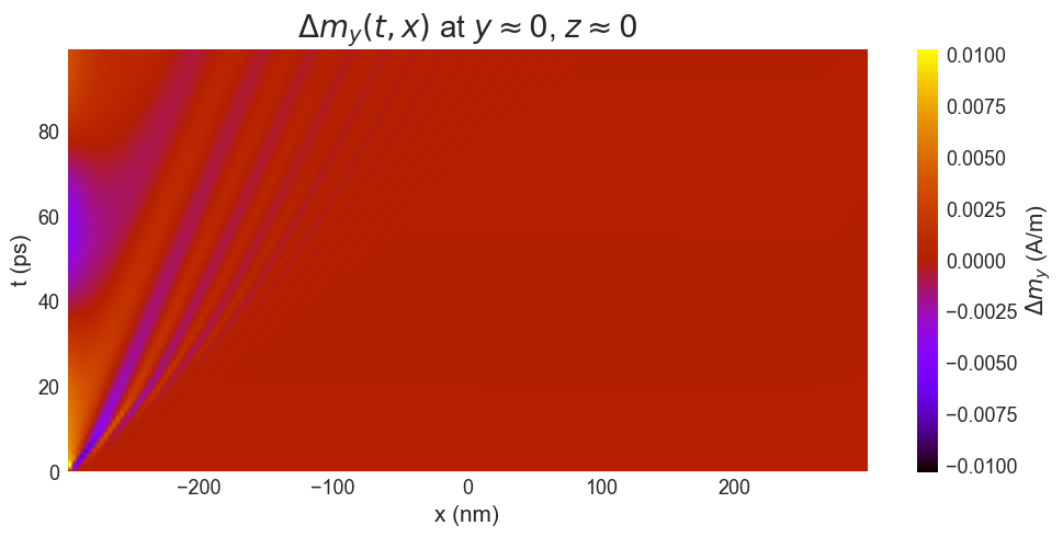 Space–time map \(\Delta m_y(x,t)\). The pulse at \(x = -300 \, \text{nm}\) launches a spin wave packet that propagates rightward. Multiple wavefronts are visible, corresponding to different group velocities (different \(k\) components). The packet reflects at \(x = +300 \, \text{nm}\) and returns, creating the characteristic diagonal striping pattern. The color scale is symmetric around zero (red = positive \(\delta m_y\), blue = negative).
The diagonal streaks in the plot directly encode the group velocity: the slope of each stripe is \(v_g = dx/dt\). Faster short-wavelength magnons appear as nearly-vertical streaks; slower long-wavelength magnons produce shallower slopes. The partial reflection at both ends and the exponential decay of amplitude over time (due to \(\alpha = 0.05\)) are both visible.
7.4 From space–time to frequency–wavevector: the 2D FFT
Why a Hanning window?
Before Fourier transforming, we multiply \(\Delta m_y(x,t)\) by a Hanning (raised cosine) window in both dimensions:
win_t = np.hanning(n_steps + n_pulse)[:, np.newaxis]   # (Nt, 1)
win_x = np.hanning(nx)[np.newaxis, :]                   # (1,  Nx)
dm_y_w = dm_y * win_t * win_x
The Hanning window tapers the signal smoothly to zero at both ends. Without it, the abrupt truncation of the signal at the boundaries causes Gibbs ringing: spectral energy “leaks” from high-amplitude frequencies into neighboring bins, blurring the dispersion curve. The Hanning window costs a factor of ~2 in frequency resolution (because it broadens each spectral peak), but eliminates the leakage almost entirely. For a dispersion relation measurement, sharp localization in \((\omega, k)\) space matters more than absolute resolution.
2D FFT
fft2d   = np.fft.fftshift(np.fft.fft2(dm_y_w[:, ::-1]))
fft_mag = np.abs(fft2d) / ((n_steps + n_pulse) * nx)
Two subtleties:
[:, ::-1]reverses the spatial axis before the FFT. The physical convention is that positive \(k\) corresponds to rightward propagation (increasing \(x\)). Without this flip, the sign of \(k\) in the plot would be reversed.np.fft.fftshiftrecenters the output so that zero frequency (and zero wavevector) is at the center of the array, giving a \((\omega, k)\) map symmetric around the origin.- Division by \(N_t \times N_x\) normalizes the FFT amplitude to be independent of array size.
Frequency and wavevector axes
dt = save_dt
dx = drive_eq[0].mesh.cell[0] * 1e9       # cell size in nm

# Nyquist frequency: f_max = 1/(2·dt) = 1 THz → 1000 GHz
omega_GHz = np.fft.fftshift(np.fft.fftfreq(n_steps + n_pulse, d=dt)) * 1e-9

# Nyquist wavevector: k_max = π/dx = π/3 rad/nm ≈ 1.05 rad/nm
k_per_nm  = np.fft.fftshift(np.fft.fftfreq(nx, d=dx)) * 2 * np.pi
np.fft.fftfreq(N, d=dt) returns frequencies in Hz with Nyquist frequency \(f_N = 1/(2\Delta t) = 1 \, \text{THz}\). Multiplying by \(1 \times 10^{-9}\) converts to GHz. For the wavevector, fftfreq returns \(k / (2\pi)\) in units of \(\text{nm}^{-1}\); multiplying by \(2\pi\) gives \(k\) in rad/nm.
8. Results
8.1 Dispersion relation
We plot only the positive-frequency half (the negative-frequency half is the complex conjugate and carries no new information):
pos    = (omega_GHz >= 0) & (omega_GHz <= 500)
extent = [k_per_nm[0], k_per_nm[-1], omega_GHz[pos][0], omega_GHz[pos][-1]]

fig, ax = plt.subplots(figsize=(8, 6))
im = ax.imshow(fft_mag[pos, :], aspect='auto', origin='lower',
               extent=extent, cmap='gnuplot')
ax.set_xlabel(r'$k$ (rad/nm)')
ax.set_ylabel(r'$\omega$ (GHz)')
ax.set_title('Spin wave dispersion relation')
plt.colorbar(im, ax=ax)
plt.tight_layout()
plt.show()
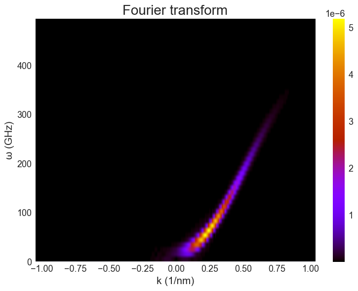 Dispersion relation \(\omega(k)\) obtained by 2D FFT of the space–time data. The bright ridge is the spin wave branch. The parabolic shape at large \(k\) confirms the exchange-dominated regime \(\omega \propto k^2\). At small \(k\), the curve flattens due to the magnetostatic (dipolar) contribution — the finite-radius correction shifts the dispersion upward at long wavelengths.
8.2 Physical interpretation
The bright ridge in the \((\omega, k)\) plane is the spin wave dispersion relation. Several features are visible:
Parabolic branch (large \(k\)): At wavevectors \(k \gtrsim 0.2 \, \text{rad/nm}\), the dispersion follows \(\omega \approx (2A\gamma_0/\mu_0 M_s) k^2\). Using our parameters:
\[\frac{2A\gamma_0}{\mu_0 M_s} = \frac{2 \times 13 \times 10^{-12} \times 2.211 \times 10^5}{4\pi \times 10^{-7} \times 0.86 \times 10^6} \approx 5.3 \, \text{nm}^2 \cdot \text{GHz}\]So at \(k = 1 \, \text{rad/nm}\): \(\omega \approx 5.3 \, \text{GHz} \times (1 \, \text{nm})^{-2} \times (1 \, \text{nm})^2 \approx 5.3 \, \text{GHz}\). Wait, let me recalculate in consistent units:
\[\omega(k) \approx \frac{2 \times 13 \times 10^{-12} \times 2.211 \times 10^5}{(4\pi \times 10^{-7}) \times 0.86 \times 10^6} k^2\]At \(k = 0.5 \, \text{rad/nm} = 5 \times 10^8 \, \text{rad/m}\): \(\omega \approx 5.3 \times 10^{-15} \, \text{m}^2/\text{s} \times (5\times 10^8)^2 \approx 1.3 \times 10^{11} \, \text{rad/s} \approx 21 \, \text{GHz}\)
This is consistent with the scale visible in the dispersion plot.
Flat region near \(k = 0\): The dispersion flattens and acquires a finite frequency at \(k = 0\), the ferromagnetic resonance (FMR) frequency of the nanowire. This arises from the transverse demagnetizing field: even a uniform (\(k=0\)) precession costs energy because the circular cross-section has \(N_y = N_z \approx 0.5\), creating a restoring force.
Symmetric branches at \(\pm k\): The spectrum is symmetric around \(k = 0\). This is because the pulse excites spin waves traveling in both directions (toward \(+x\) and \(-x\)), and after reflections at both ends, the wire supports standing-wave patterns that contribute both \(+k\) and \(-k\) components.
8.3 Connection to experiment
This computational method is the direct analogue of Brillouin light scattering (BLS) spectroscopy, the primary experimental technique for measuring spin wave dispersion in nanomagnets. In BLS, an incident laser beam inelastically scatters off magnons, gaining or losing their energy and momentum. By varying the laser angle (and thus the transferred wavevector \(k\)) and measuring the frequency shift, one traces \(\omega(k)\) point by point. Our simulation gives the full dispersion curve in a single run.
9. Summary
| Step | Code | Physics |
|---|---|---|
| Mesh | df.Region + df.Mesh, cell 3×1×1 nm³ | Must resolve \(\ell_\text{ex} = 5.3\) nm |
| Cylinder mask | Ms_fun + valid="norm" | Shape anisotropy → single-domain ground state |
| Relaxation | mc.MinDriver, \(\alpha = 0.5\) | Overdamped → no oscillations, fast convergence |
| Pulse | 1 ps, 100 kA/m, one-cell-wide at left end | Broadband \(k\)-spectrum via spatial localization |
| Dynamics | mc.TimeDriver, \(\alpha = 0.05\), 200 ps | Spin waves propagate, reflect, decay slowly |
| Space–time | \(\Delta m_y(x,t)\), 400 snapshots | Visualize group velocity and reflections |
| 2D FFT | Hanning window + np.fft.fft2 | Spectral leakage suppressed; \(\omega(k)\) extracted |
The workflow generalizes immediately: change Ms_fun to any geometry (disk, rectangle, ring), add a bias field via mm.Zeeman, or include magnetocrystalline anisotropy via mm.CubicAnisotropy or mm.UniaxialAnisotropy. The 2D FFT method is universal — it is the standard approach for measuring spin wave spectra in micromagnetic simulations and directly comparable to BLS and vector network analyzer (VNA-FMR) experiments.